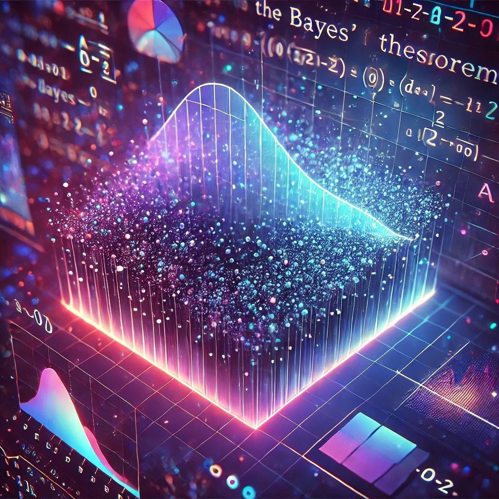
The Bayes Classifier: The Gold Standard of Classification

Explore the theoretical foundations and practical limitations of machine learning's most optimal classifier, and understand why it remains an important benchmark in the field.

"AI Disruption" publication New Year 30% discount link.

---

Hi, I'm

Giulio Donninelli

, a Data Science student at Bicocca University of Milan with a deep passion for Machine Learning and AI. I created this blog to refine my understanding of key concepts and share insights with others. Whether it’s a short lesson on fundamental AI techniques, a breakdown of research papers, or updates on my projects, my goal is to make complex ideas more accessible. If you're interested in Machine Learning, and Statistics, you're in the right place!

When it comes to classification tasks, every model strives to minimize errors. But what if we had a theoretical baseline—a classifier so optimal that no other method could outperform it? Enter the Bayes Classifier. While it’s often impractical to implement directly, it serves as the benchmark against which all other classifiers are measured.

In this post, we’ll explore:

• What the Bayes Classifier is and why it’s theoretically optimal

• How it leverages posterior probabilities

• The decision rule follows

• Why it’s often impossible to use in practice

• The classifiers inspired by it (Naïve Bayes, LDA, etc.)

• A Python snippet to approximate Bayes Classification

Let’s dive in.

The Foundation: Minimizing Classification Error

In any classification problem, we aim to assign an observation to the class with the highest probability, given our knowledge. Mathematically, this is expressed as:

\( P(Y=j|X) \)

where we select the class that maximizes this probability.

The expected classification error rate (EPE), analogous to the expected prediction error in regression, measures how often a classifier mislabel an observation. The Bayes Classifier minimizes this error, achieving what’s known as the Bayes rate—the lowest misclassification rate possible for any given dataset.

This is why all classifiers, from logistic regression to deep learning models, aspire to approximate the Bayes Classifier.

The Bayes Decision Rule

Given a new observation

\(\gamma\)

with feature vector X, the Bayes classifier assigns it to the class with the highest posterior probability:

\(Y(\gamma)=\arg\max_jP(Y=j|X) \)

Using Bayes’ Theorem, we express this posterior probability as:

\( P(Y=j|X)=\frac{P(X|Y=j)P(Y=j)}{P(X)} \)

where:

• P(X|Y=j) is the likelihood of observing a given class,

• P(Y=j) is the prior probability of class,

• P(X) is the marginal probability of.

To classify a new observation, we compute these probabilities and assign it to the class with the highest posterior probability.

Decision Rules: MAP and Likelihood Ratios

The Bayes classifier can be framed through different decision rules, each with its own interpretation and use case.

1. Maximum A Posteriori (MAP) Rule

This is the fundamental decision rule of the Bayes Classifier:

\(Y(\gamma)=\arg\max_jP(Y=j|X) \)

It selects the class with the highest posterior probability, making it a direct application of Bayes’ theorem in decision-making.

2. Likelihood Ratio Test (LRT)

A reformulation of the MAP rule isolates the likelihoods:

\(\frac{P(X|Y=1)}{P(X|Y=2)}\ge\frac{P(Y=2)}{P(Y=1)} \)

If the ratio of likelihoods exceeds the ratio of prior probabilities, the observation is assigned to class 1; otherwise, it is assigned to class 2. This test is particularly useful in statistical hypothesis testing where prior information is incorporated.

3. Maximum Likelihood (ML) Decision Rule

If we assume equal priors (i.e., both classes are equally likely), we simplify to:

\( \frac{P(X|Y=1)}{P(X|Y=2)}\ge1 \)

This means we classify based solely on which class is more likely to be given X without considering prior probabilities. This rule is commonly used when no prior knowledge about class distributions is available.

These decision rules form the backbone of Bayesian classification and serve as guidelines for constructing more practical classifiers.

The Limits of the Bayes Classifier

So, why don’t we always use the Bayes Classifier if it’s optimal?

• We don’t know the true distributions. The posterior probability requires knowledge of the likelihood function P(X|Y), which is usually unknown.

• Computational constraints. Even if we approximate these distributions, computing exact posterior probabilities for high-dimensional data can be infeasible.

• Real-world data is noisy. The Bayes Classifier assumes perfect knowledge of distributions, which is rarely the case in practical applications.

Because of these limitations, we turn to approximate methods inspired by the Bayes Classifier.

Practical Approximations

Several practical approximations of the Bayes Classifier aim to balance accuracy and computational efficiency. Two notable methods are Naïve Bayes and Linear Discriminant Analysis (LDA), which provide simplified models for real-world classification tasks.

I've discussed these methods in detail in dedicated posts on my blog rather than covering them here. If you're interested in how they work and how they compare, check out my post on Naïve Bayes and LDA to learn more.

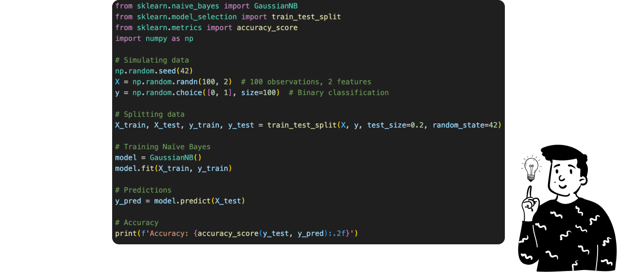
A Simple Python Implementation

Here’s a quick example of Naïve Bayes in Python using Scikit-Learn:

Conclusion

The Bayes Classifier represents the theoretical gold standard for classification, minimizing misclassification rates by leveraging posterior probabilities. However, its reliance on unknown distributions makes it impractical in most real-world scenarios.

Naive Bayes: The Simple Algorithm That Keeps Beating the Odds